Collecting and Creating Bathymetric Maps with the BlueBoat and Ping2

Introduction

Basic hydrographic surveys are easy to do with the Ping2 and BlueBoat, and unlike with a traditional chartplotter, you can review the data as it comes in! This guide assumes your Ping2 is mechanically and electrically connected on the BlueBoat, and you’ve confirmed normal operation with the Ping Viewer software based on the integration guide. In this guide, you’ll learn how to install a simple extension to help collect survey data, and how to use free and open source software to create maps. Let’s get started!

Software Setup

Make sure you’ve completed the software setup for the Ping2 before proceeding. To visualize and format collected data more effectively and conveniently, we created a simple extension that saves data locally on the boat and displays it live when connected! Autopilot log files without confidence information and a desire to create a more involved example of a BlueOS extension combined to motivate development of this extension!

If you’d like to report an issue, contribute with a pull request, or fork the extension, we’re excited to see where development leads!

Simple Ping2 Survey Extension: Installation

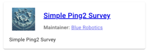
Navigate to the Extensions menu on the left side of the page, select Blue Robotics as the Provider, and find Simple Ping2 Survey in the list. You will only see options here if your Raspberry Pi running BlueOS connects to WiFi with internet access. Select the extension and press the install button.

Within a couple minutes of finishing the installation, this icon will appear in the BlueOS menu:

You can also load the page full-screen, by clicking the Webpage URL next to the SimplePing2 service in the Available Services menu (accessed in Pirate Mode.)

UI Overview

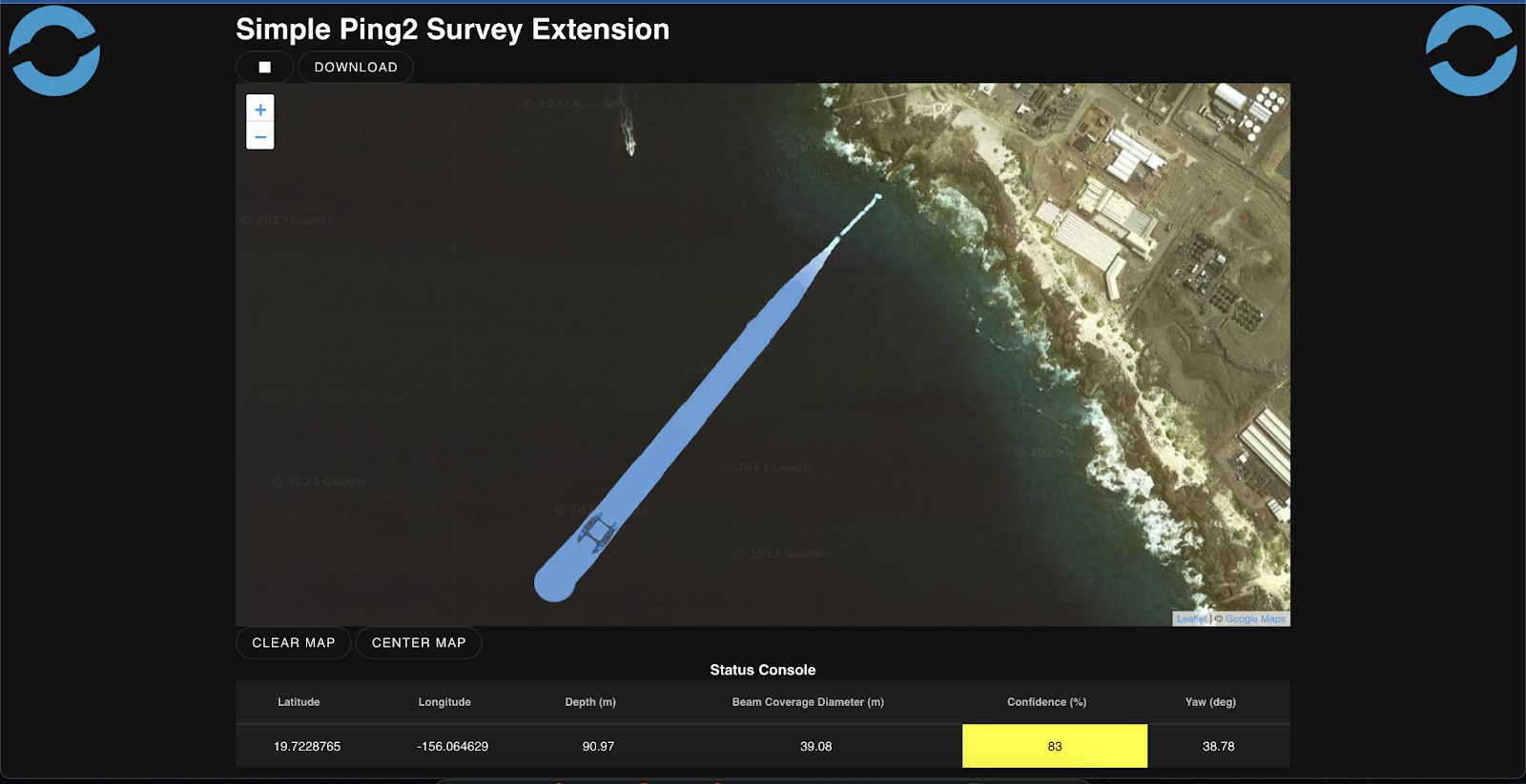
The Simple Ping2 Survey Extension tries to live up to its name. To record and view data, click the triangular play button in the upper left. To stop logging data and updating the map, click the stop icon that replaces play. At any point, click Download to receive all logged data. The Clear Map button only clears displayed data.

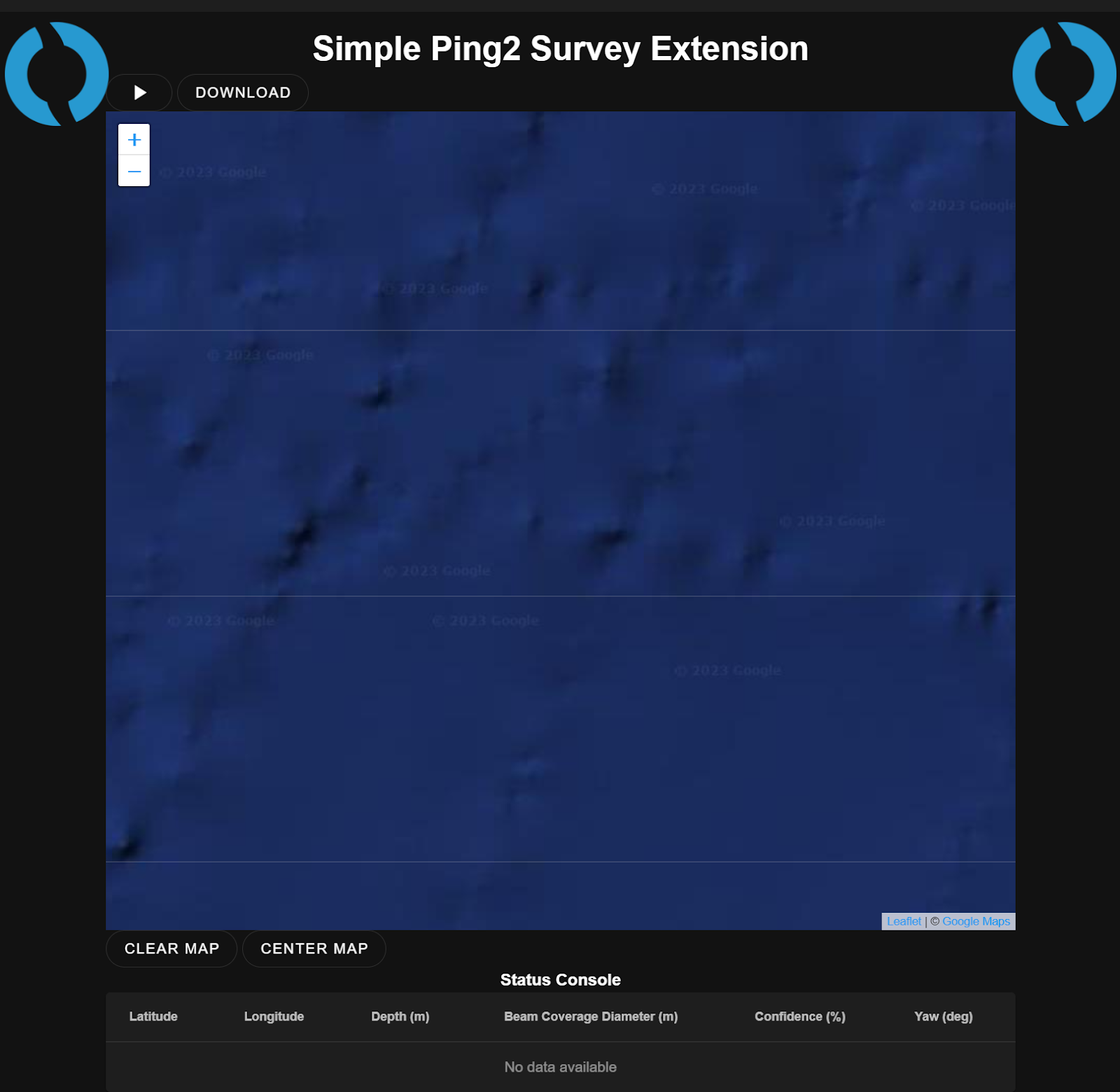
The map shows the position and orientation of the BlueBoat. If the confidence of the Ping2 Depth measurement is above 95%, a colored circle appears on the map. The depth is indicated by the shade of the color, and the diameter is a to-scale representation of the beam coverage diameter. This is based on the 25 degree beam of the device, and indicates the area that is being averaged to return depth. Data is recorded at 2 Hz regardless of confidence metric or communications link onboard the BlueBoat.

The Clear Map button will clear any circles drawn on the map in the current session – this does not affect the logged data. The Center Vehicle button will center the vehicle on the map at a fixed zoom level, useful if you scroll away and get lost. The map will not center on the vehicle until the next location is received.

The Status Console updates to show a healthy connection to the vehicle, rotating the Blue Robotics logos with every other data packet received. If you lose connection to the vehicle after clicking the Play button to start logging, don’t worry about missing data! If you refresh the page and see no incoming data, clicking Play will recenter the map and continue data logging even if the GUI did not reflect it.

Field Use

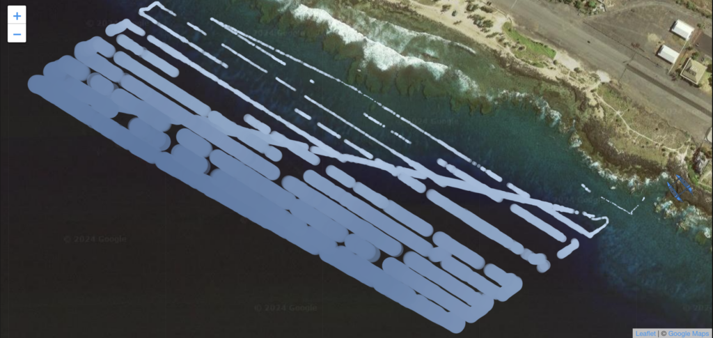
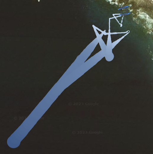
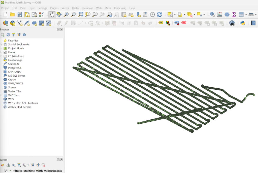
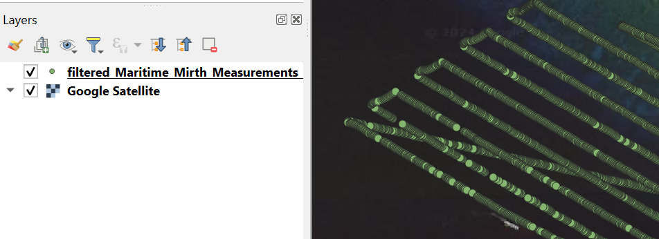
Plan and load the BlueBoat with your survey mission – you can find instructions on that process in the Operators Guide. Open the extension and click the Play button, before launching the boat. If the map centers on the vehicle, you’re ready to go! Once you’ve launched the boat, the colored circles will appear on the map indicating good readings. When you’re ready, put the boat in Auto mode and watch as it begins navigating to collect data! When you’ve finished your survey, download the file and get ready for processing. An example of a post-survey interface is shown above – the missing areas indicate times the vehicle was not connected – despite this all of the depth data was still logged!

Extension Troubleshooting

• Map tiles will only load if your computer has internet access.
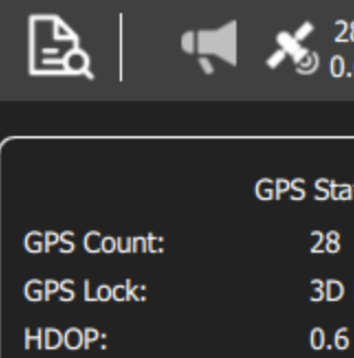
• The extension requires the BlueBoat to have GPS lock. You can find the status of the GPS in QGroundControl, but if the vehicle shows up where you expect it to on the map you are locked on!
• If operating in the field, connecting your control computer to the BaseStation with the provided USB-C cable will allow you to use a cellular WiFi hotspot to provide internet access to your computer simultaneously.
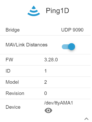
• The extension also requires the Ping2 to be detected under Ping Sonar Devices, with the MAVLink Distances turned on.

Using the data

Once you’ve downloaded the data via the Download button, it can be processed to create a map using the free and open-source software tool, QGIS. You can follow along with this section of the guide using your own data or this example data provided.

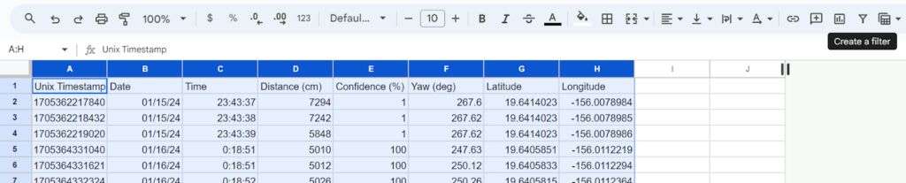
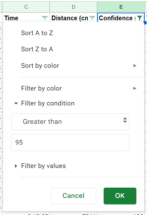
Data Selection and Quality Control 1. To filter the data, open the log file in your favorite spreadsheet application. Select all the columns, and set up a filter. 2. Configure the filter to only show rows where the Confidence value is above 95 (or whatever value you prefer). 3. After verifying the data has been filtered, copy all of it to a new spreadsheet and export/save as a .csv file, adding to the filename to signify the data is processed. This step is important to ensure your map reflects quality measurements!

Using geographic information systems software (GIS) for map creation

This type of software has existed since the 1980s and finds applications across many industries! Unlike the more commonly known (and expensive) ArcGIS, QGIS is open source Geographic Information System software. We’re not experts at using it, and developed the workflow presented here using a mix of internet research and real world testing. Considerable documentation is available for QGIS, as well as their own forum. Please don’t hesitate to reach out with feedback!

Importing the data

1. Download and install QGIS.

2. Once you’ve setup QGIS, open the program and create a new project. 3. Import the filtered data by selecting Layer, Add Delimited Text Layer. The Data Source Manager window will open, although depending on your system this can strangely open behind the main window. Once you’ve found the window, select your logfile with the .csv extension. 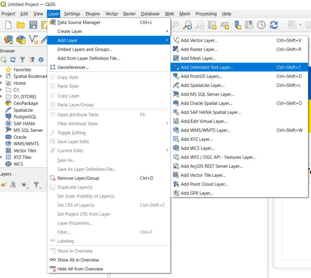4. Select the “Geometry Definition” dropdown. The X and Y field will automatically populate with the Longitude and Latitude. For the Z-Field, select Depth (cm). Select an appropriate coordinate reference system (CRS) – this refers to the standard methods of dividing up the world into coordinate spaces. This will usually be automatically selected by the location of your dataset. 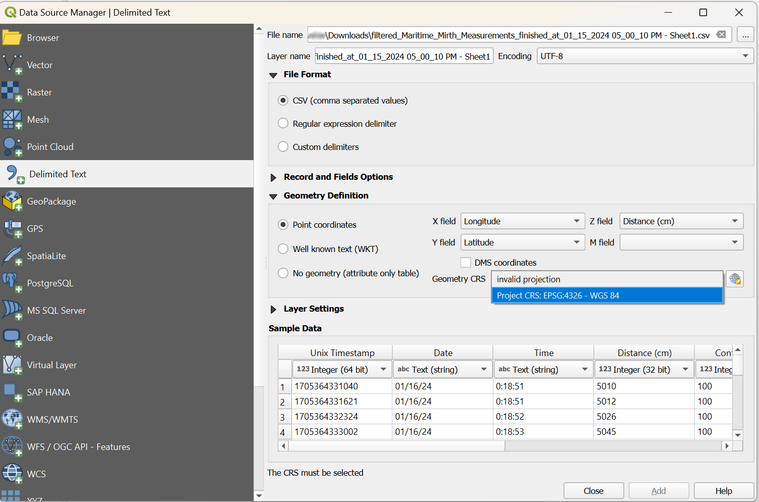5.Click add, and you will see the data points appear on the map! This is a good time to save the project. 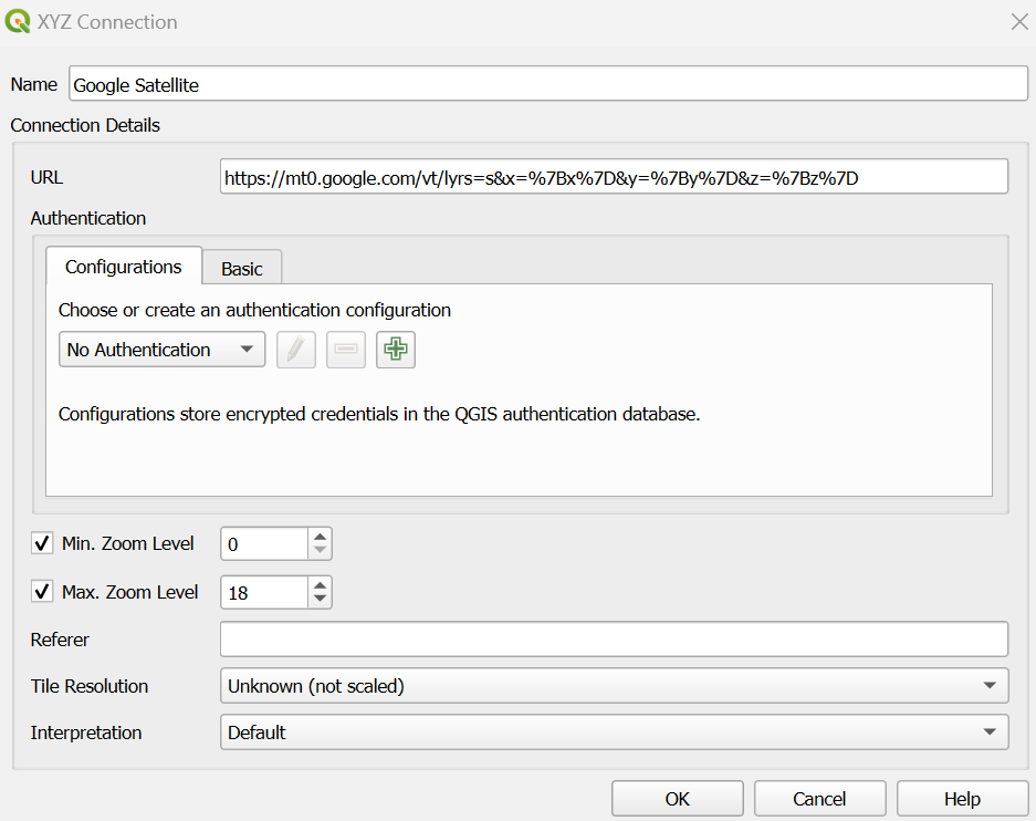6. Next, we’re going to give our map a background. In the Browser pane at top-left, right click on XYZ Tiles, New connection. Name the Connection Google Satellite and paste the following URL into the next box:

https://mt0.google.com/vt/lyrs=s&x=%7Bx%7D&y=%7By%7D&z=%7Bz%7D

7. Next, expand the XYZ Tiles section on the left and drag the Google Satellite option you created into the Layers pane below it. Your points are hidden! To fix this, drag the tile from under XYZ tiles to the bottom of the layer list, and the points will appear on top of the satellite map.

Creating a mesh

1. Adjust the zoom level by scrolling on the map so that all collected points fit nicely in the map view. Holding the Ctrl key while scrolling your mouse wheel allows for finer adjustment.

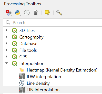
2. At the top of the QGIS window, select Processing>Toolbox.

3. Under Interpolation, double-click TIN interpolation.

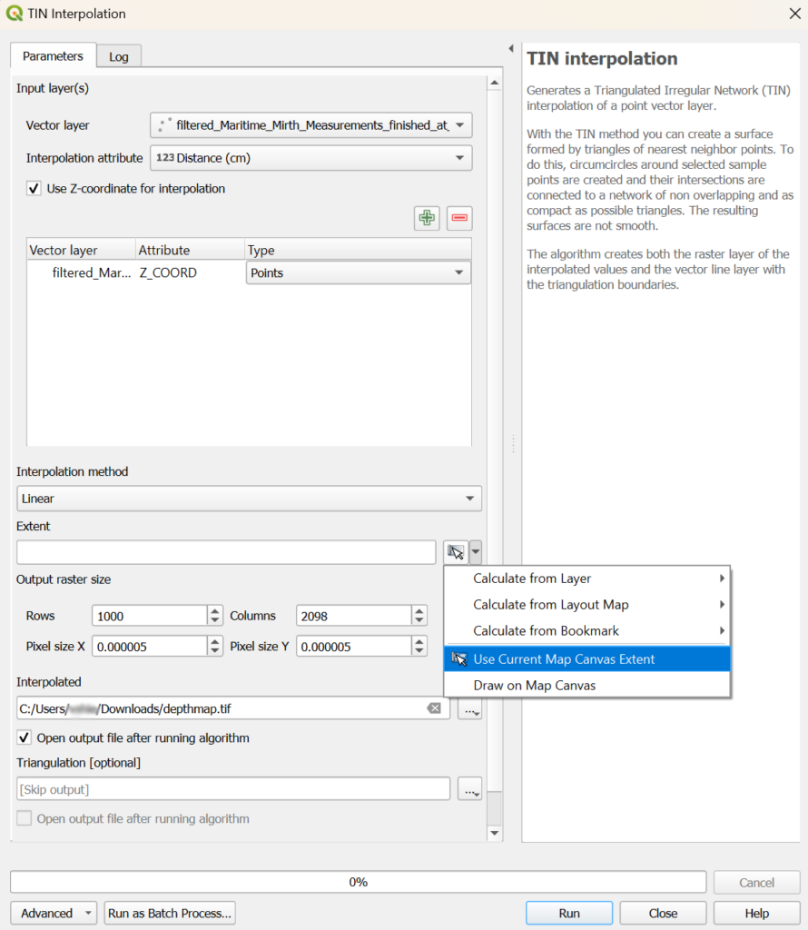
4. In the TIN Interpolation window, select the vector layer we just created with our filtered data at the top.

4A. Choose Depth (cm) as Interpolation attribute, check the box for “Use Z-coordinate for interpolation” and then click the plus button to make it appear in the list under Vector Layer.

4B. You can choose to change the Interpolation method to Clough-Toucher (cubic), but for most datasets this produces nearly identical results to Linear interpolation.

4C.For extents select Use Current Map Canvas Extent.

4D. Under Output raster size set Rows to a number > 500 (for large surveys you may want to set this higher.)

4E. Finally, to avoid weird behavior from QGIS, choose to save the output to a file (not Temporary file.)

4F. Click Run to generate the output map, which will attempt to create a surface interpolating between all the xyz coordinates in the filtered survey data.

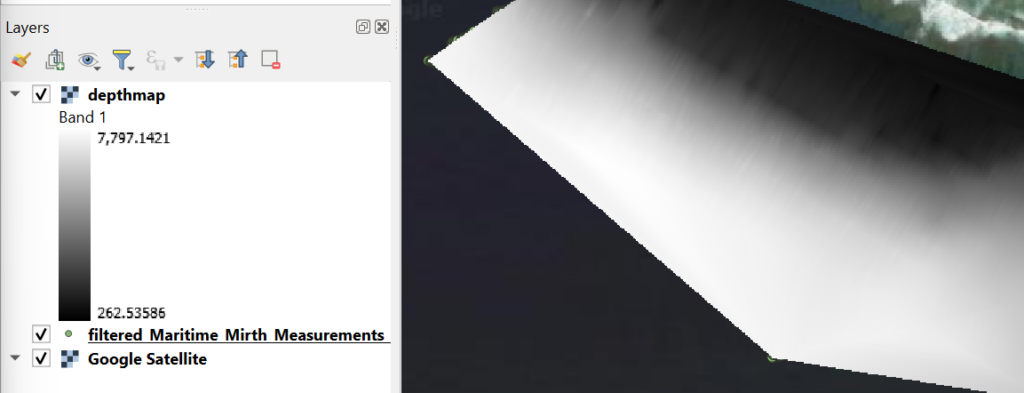
5. You can adjust the colors used to create an image that better reflects the data.

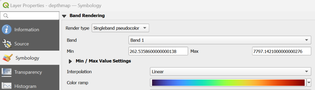
5A. Right click on the layer in the list at left, click Properties and choose Symbology in the Layer Properties window that opens. At the top, under Band Rendering, select Singleband pseudocolor.

5B. For color ramp, the “Turbo” color conveys data vibrantly, but the “Blues” option may be preferable to those with color-blindness. The range of colors will automatically be sorted between the Min and Max depth measured. 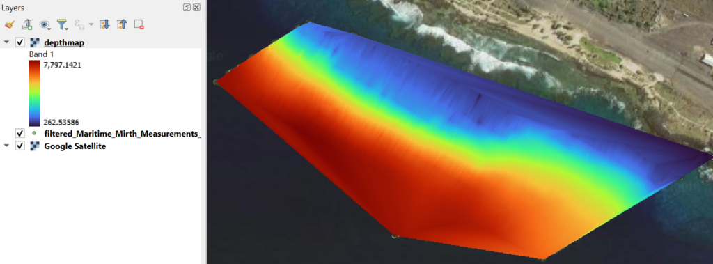6. The Transparency menu allows you to reduce the opacity of the interpolation overlay, so you can see how well it aligns with satellite imagery.

Contour maps commonly visualize terrain data, with the ground slope correlating to the closeness of the lines. Each line represents a contour of equal depth, centered between its neighbors at the chosen elevation interval. Follow these steps to generate this map layer:

Extracting a contour plot

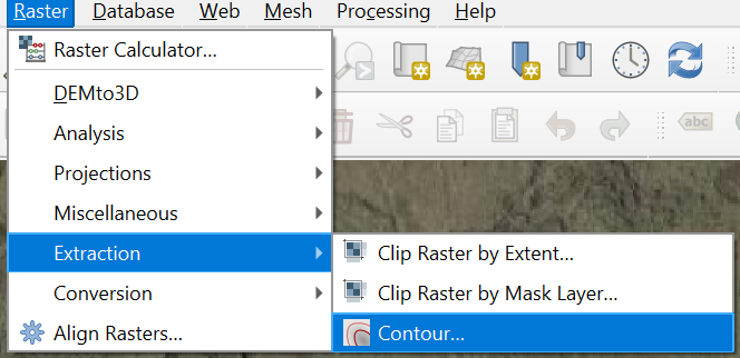
1. From the top menu select, Raster, Extraction, Contour.

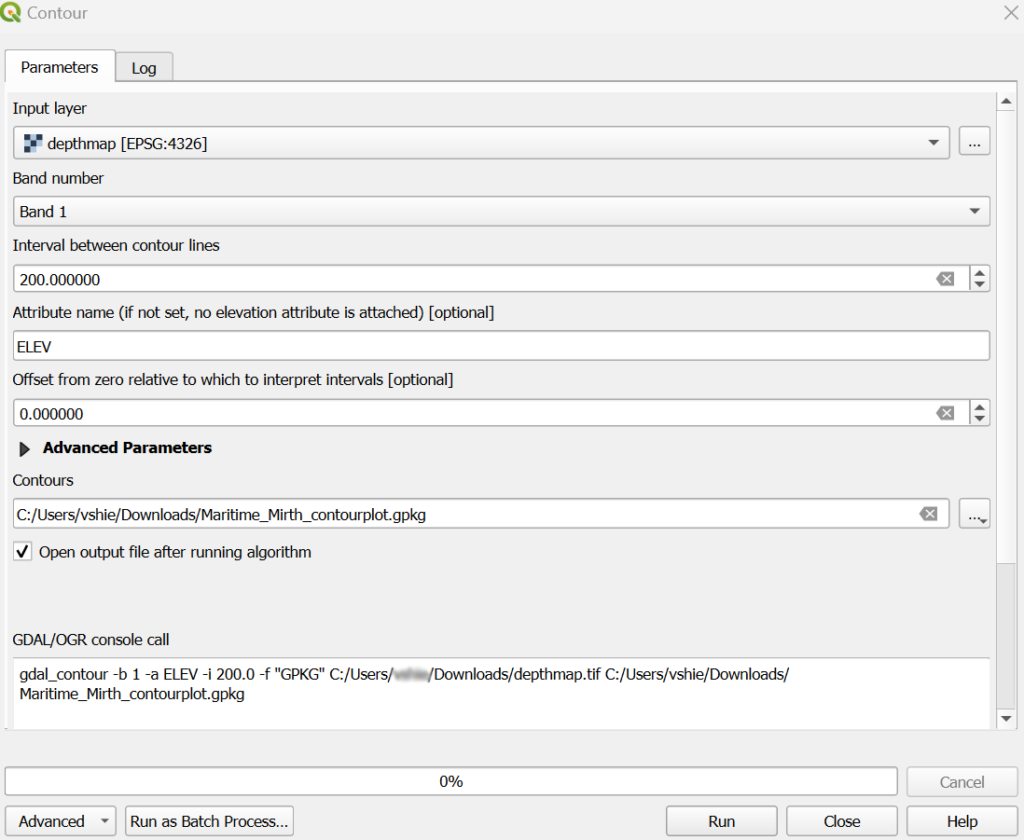
2. Verify that you have set the Input layer to the interpolation map created in the previous step. Set the interval between contour lines – remember to note the units! Since the raw data is in centimeters, generate a map with a 2 m, or 200 cm, vertical separation between contour lines. Create an output file to save this contour map, as QGIS can behave unpredictably with temporary files. Click Run to generate the plot.

3. The plot lines can be adjusted and labels set up by right clicking on the layer and selecting properties, or double clicking the layer. For line color, chosen under Symbology – we prefer yellow #fedd00.

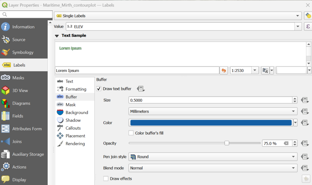
4. Under Labels, select Single Labels and choose ELEV for the Value to display. Green #7ac943 is a good choice for text that will show up on most satellite water backgrounds. A Buffer and Mask can both help make the labels more readable. Enable and set Buffer size to 0.5 mm, and use Blue #135ea4 for the color. Set the Buffer to 75% opacity. Enable and set Mask Size to 0.4 mm, with 100% opacity. 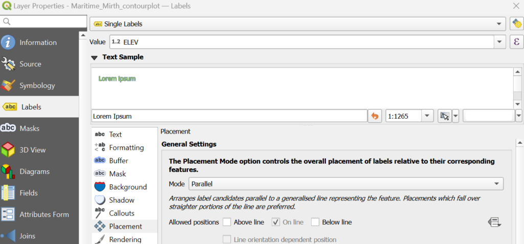Under Placement, Check the “On line” box and uncheck the “Above line” box. [/list]

Reviewing the data

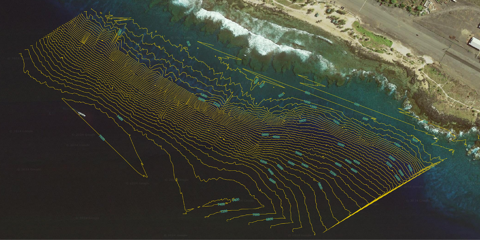
Here is the completed map! In QGIS, as you zoom in, the system automatically shifts the contour labels to the center of the visible portion of each line. When designing your survey, it is important to plan transects at 90 degrees with good overlap, and space them out at an appropriate interval for the depth and type of terrain! 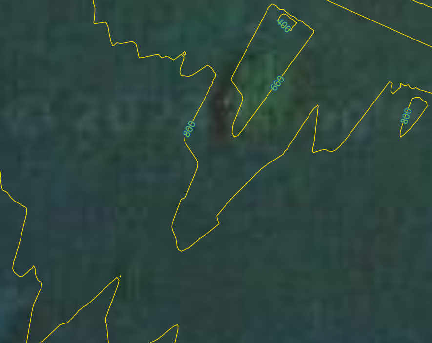The contour lines can go a bit funny at the edges of our plot, this is expected. You can see we correctly found this coral head!

More Things to Try

Volume measurement

Using single-beam survey data to determine the volume of a small body of water, such as a reservoir or pond, is a common application. You can easily accomplish this with your contour plot and a few additional steps. In the interest of brevity, check out this great video that details the process!

3D Model export for 3D printing

You can generate a 3D model from the TIN layer created with just a few clicks! This great plugin for QGIS makes the process easy, and even lets you split a model up into multiple chunks. You can learn how to do that with this handy resource!